Researching age-related decline

It is common sense that not only physical but also mental abilities decline with ageing. When chess players talk about it, they often mention the former world championship challenger Viktor Korchnoi. He experienced his second heyday at the age of 68 in 1999, when he was ranked number 16th in the world, only 20 points below his all-time high of 2,695 Elo points. Other examples are the former chess world champions Vassily Smyslov, who played the candidates final in 1984 at the age of 63, and Emanuel Lasker, who won the famous New York 1924 tournament at the age of 56. Physical abilities decline faster than mental abilities. We do not find 60-year-old athletes in Olympic track and field events.

Chess is sometimes dubbed the “drosophila (fruit fly) of cognitive psychology”, because it provides a reliable measure of skill, the Elo rating system (Elo, 2008, originally published in 1978), and large databases for longitudinal studies. Chess players are rated on a continuous scale which ranges from about 1,000 Elo points for beginners to about 2,800 points for the best international grandmasters. Age-related decline in chess has been a subject of scientific research. The inventor of the Elo system – Arpad E. Elo – found that “the average peak is about 120 points higher than the level at ages 21 and 63” (Elo, 2008, p.93). Roring & Charness (2007) criticized the fact that Elo had analysed only 36 elite players. They based their regression analysis on FIDE (the World Chess Federation) players of different strength, finding that “ageing was slightly kinder to the initially more able, who showed milder decline past their peak” and that “tournament activity had smaller effects on rating for older adults”. They used the quadratic function to fit the curves.

Vaci, Gula & Bilalić (2015) contradicted Roring & Charness’s findings. They compared German and FIDE expert and non-expert players, and used the cubic function to fit the curves. They argued that the quadratic function was not “the best choice” and that the FIDE database would suffer “from serious methodological problems”. Only the superior German database would guarantee correct results. They found “ proportionality between prepeak increase and postpeak decrease”, but that experts’ decline started to stabilize earlier, and “the more players engaged in playing tournaments, the less they declined and the earlier they stabilized”. Vaci et al. (2015) explained chess trajectories based on the model of career trajectories of Simonton (1997), who described the change in the creative productivity of famous composers, painters, scientists, and writers across their entire life span through an exponential mathematical function. He defined creative productivity as the number of compositions, paintings, patents, or publications. Simonton found that the more steeply that his protagonists rose to the peak, the faster they subsequently declined, and that the curves approached the “zero-output rate asymptotically”. Vaci et al.’s (2015) curves in their Figure 5 B were obviously similar to Simonton’s (1997) Figure 1.

It is shown in the first part of the current study that Vaci et al.’s (2015) paper was an example of the often-cited “replication crisis” (Open Science Collaboration, 2015) in the social sciences. The second part explains how their model has to be changed to work correctly. The thirdsection presents the German and FIDE players’ correct chess trajectories across the entire life span and the true influence of tournament activity. Links to the original papers are provided in the reference section.

Vaci et al.’s (2015) mysteries

Asymmetric Cubic Functions. When I saw Vaci et al.’s (2015) curves in their Figure 5 B, I remembered what I had learned at school a long time ago, namely that all cubic functions are rotationally symmetrical about their inflection point. However, the authors’ curves – which are copied in Figure 1, and can also be seen in Vaci & Bilalić (2017), Figure 2 – are not. The authors offered their German and FIDE database for download, so it was possible to re-analyse their study based on the original data. Figure 1 presents the true curves obtained by Vaci et al.’s (2015) models 1 and 2. They show the typical late cubic rise as a consequence of the built-in symmetry of cubic functions. Vaci et al. (2015) eliminated it in an unknown way.

The authors’ model 2 differed from their model 1 by including the categorical variable ability, comprising the sub-groups of experts and non-experts, which should only enable the analysis of both skill groups in one run but otherwise not change the result. Instead, the curves of model 1 are completely different, and the non-experts overtake the experts at about 58 years of age (Figure 1). I will explain the reasons in the ‘ Extrapolation Error’ sub-section. It is obvious that the authors based their results on their model 2.

Simonton (1997, p. 71) called the replacement of his exponential formula by the cubic function “theoretical nonsense” due to the late cubic rise. Vaci et al. (2015) thanked Simonton for his comments on a previous draft in their acknowledgement. Did he forget to tell them that they had conducted “theoretical nonsense”? Simonton (1997, p. 84) mentioned the “swan-song phenomenon” in classical music, whereby famous composers had an upsurge of creativity shortly prior to death, although this remains unknown for chess players thus far.

Experts Who Were Non-Experts. The authors stated that their “expert group consisted of players with a peak rating of 2,000 points or more, while all other players were defined as non- expert players”. This is the usual definition. The German expert curve in Vaci et al. (2015), Figure 5 B, shows a maximum slightly below this margin, which is actually impossible. The re-analysis revealed that from a total of 40,617 expert players (marked as “Ability 2” in the database), only 12,535 were real experts, whereas 28,082 players were non-experts with peak ratings between 1,723 and 1,999 points. This was not a simple oversight. In the FIDE database, from a total of 66,435 players in the non-expert group, only 35,413 players were real non-experts whereas 31,022 players were experts with peak ratings up to 2,166 points. The non-experts’ mean rating in the FIDE database was considerably higher than the experts’ mean rating in the German database (1,982 versus 1,843 points). This made no sense, as Vaci et al.’s (2015) study was designed to compare equally-skilled players in both databases, although in this way the authors could confirm Roring & Charness’s (2007) finding that age was kinder to those who were more able in the FIDE database.

Imaginary Probability Density Functions. Vaci et al.’s (2015) intention was to discredit the FIDE database for the following reason. Bilalić, Smallbone, McLeod & Gobet (2009) had analysed the German database and explained gender differences in chess based on a participation rate hypothesis. Howard (2014) claimed instead that natural talent makes the difference, basing his results on the FIDE database. Vaci, Gula & Bilalić (2015) countered and argued that the FIDE database “suffers from serious methodological problems”, and that “studies with restricted FIDE data regularly find differences between women and men in skill”. It has recently been shown how Bilalić et al. (2009) evoked the illusion of a common distribution of male and female rating values (Wiesend, 2019).

The probability density curves presented in Vaci et al. (2015), Figure 1 and Vaci & Bilalić

(2017), Figure 1 seem to prove that the FIDE database is only a small subset of the German database. The blue and red lines in Figure 2 show the correct rating density curves. The total area under density curves (AUC) is always 1.0, corresponding to a probability of 100 per cent. Hence, if two density curves are plotted in the same graph, their AUCs must be identical. Instead, the authors’ AUC of the German database in their Figure 1 A is twice as large as that of the FIDE. The German curve peaks at 2,025 points, while the calculated mean is 1,603 points. The curve was obviously shifted to the right by about 400 points.

Vaci et al. (2015) falsely stated in their legend to their Figure 1 A: “The only overlap between them is at the highest values of the German database and the lowest values of the FIDE database.” The same sentence can be found in the legend to Vaci, Gula, & Bilalić (2014), Figure 1, where the probability density curves are closer to reality. Vaci et al. (2015) wanted to emphasize the restricted rating range of the FIDE database, whereas Vaci et al. (2014) stressed the differences between the two databases. For every occasion the most suitable curves!

How Vaci et al.’s (2015) model has to be changed to work correctly

Extrapolation Error

Vaci et al. (2015) used the open source software R (R Core Team, 2020) and mixed-effect modelling implemented in the R package ‘lme4’ (Bates, Maechler, Bolker, & Walker, 2015) to calculate the relationship between the independent variables (also called fixed effects or predictors) age, games and stale, and the dependent variable rating. Stale was a measure for inactivity, defined as the number of years that players had played no tournaments.

If a player has multiple observations due to having played more than one tournament, then the ratings are not independent but correlated, because every player has her/his individual skill level. Therefore, in a first step individual skill trajectories have to be fitted by including random effects. The term mixed-effect modelling stands for the combination of fixed and random effects.

Equation 1 shows the individual regression equation for the authors’ basic model without the additional variables games and stale. Databases list the players’ year of birth. Age is thus the difference between the year in which a player’s rating was recorded and her/his year of birth. The ‘x’ is the multiplication sign.

(1)

The software computes the regression coefficients β. The red terms in Equation 1 are the individual part, which is different for each player. The first term is called random intercept, the second one random slope. The blue terms are the general part, which is identical for each player. Age is included as the first, second and third power, because the third-degree polynomial or cubic function is used for curve fitting.

The German database that Vaci et al. (2015) used in their study listed 119,785 players, although 49,386 of them had been active for only five years or less, and none of them for 20 years or longer. In order to calculate trajectories from 10 to 80 years of age, the model is forced to estimate the missing data by extrapolation, which is shown in Figure 3 for three players. Long- distance extrapolation is flawed, and the estimated ratings are unrealistic. The curves of all 119,785 players in the database are extrapolated in this way. The overall curve is calculated as the mean of the 119,785 extrapolated curves at any time point or age. The regression equation of the overall curve is shown in Equation 2.

(2)

Compared with Equation 1, only the individual part has changed. It is transformed into the mean of all of the players’ random intercepts. The random slope term has disappeared, because the software

is programmed in such a way that the mean of all individual random slopes is always zero. Thus, the slope of each player is influenced by the slopes of all other players. Consequently, the extrapolation is different for the authors’ models 1 and 2, while the goodness of fit – which measures the distance between the fitted curve and the data points – is the same (see Figure 3). This is the reason why the authors’ models 1 and 2 lead to different results, as shown in Figure 1.

In other words, Vaci et al.’s (2015) models combining random intercept and random slope were inappropriate, because the periods in which the players were active were too short. This was one of their cardinal errors. They considered only the goodness of fit (see their Figure 3) but not the extrapolation error.

Effect of Additional Variables

Equation 3 shows the German database’s regression equation, obtained with Vaci et al.’s (2015) model 1, when the authors’ regression coefficients given in their Table 2 are entered. Games and age are interacting.

Rating = 597.1 + 97.3 x Age – 2.539 x Age² + 0.0186 x Age³ + 2.55 x Games – 8.743 x Stale – 0.135 x Age x Games + 0.0026 x Age² x Games – 0.00001 x Age³ x Games

(3)

In order to plot this function in the two-dimensional age-rating plane, it is necessary to enter concrete games and stale values. It makes sense to take the means. Cubic curves are only obtained if the same games and stale values are entered at any age. Different values result in 71 separate data points, one for each year between 10 and 80. In the case of the German database, the 71 data points were located on the cubic curve, because the variability of the games and stale values was rather small. Vaci et al. (2015) calculated the inflection points of their curves “by setting the second derivative of the estimated model equation to zero”, so they must have used continuous functions and not point-by-point products. However, the curves in Vaci et al. (2015), Figure 4 B and Figure 5 B show small kinks at around 45 years of age, which are unusual for differentiable functions.

If the categorical variable ability is included interacting with age and games — as in Vaci et al.’s (2015) model 2 — the total number of terms increases from 9 to 17. The terms and coefficients are presented in the authors’ Appendix C. This is seemingly what they meant when they determined “the best and most parsimonious model”. My understanding of this principle — which is known as “Occam’s razor” — is quite different: if the task is to calculate an overall curve in the age-rating plane, then only these two variables are needed. Games and stale must be estimated, which is inaccurate in a strictly scientific sense. Thus, it is much better to leave them aside.

Seventh-Degree Polynomial and Random Intercept Alone

Chess trajectories are characterized by a steep onset and a long plateau phase. The cubic function is unable to fit such data. It is restricted in its shapes, and not sufficiently flexible. Higher-degree polynomials are needed, which were tested starting from the fourth degree. The curves approached a final shape that remained unchanged from the seventh to eight degree. The seventh degree was thus the suitable choice.

The extrapolation error was caused by the random slope. If random intercept is used alone, the software avoids the flawed individual extrapolation. In a first step, it calculates a prototypical function ranging from 10 to 80 years, which is suitable for every player. This function is parallelly shifted by different intercepts to fit the individual curves. Each player thus has the same extrapolated curve shape. In case of the German database, R squared — which is a measure of goodness of fit and lies between 0 and 100% — was 97.3 % for Vaci et al.’s (2015) model 2, and 95.4 % for the model with seventh-degree polynomial and random intercept alone (hereafter RI7), which is still sufficiently good. The slightly better fit is paid dearly by the flawed extrapolation.

Equations 4 and 5 show the R code and the regression equation of model RI7. The term (1|ID) in the R code shows that random intercept alone (RI) is used, while (1+Age|ID) would indicate random intercept and random slope combined (RIS). ID is a column in the dataset that specifies the players’ identification numbers. The function ‘lmer’ is part of the ‘lme4’-package (Bates et al., 2015) in R.

RI7 <- lmer (Rating ~ poly (Age, degree=7, raw=T) + (1|ID), data=dataset)

Rating = β₀ + β₁ x Age + β₂ x Age² + β₃ x Age³+ β^₄ x Age⁴ + β₅ x Age⁵ + β₆ x Age⁶ + β₇ x Age⁷

⁽⁵⁾

Figure 4 presents the real experts’ observations in the German database as a cloud of small grey circles, and shows that only the curve obtained with model RI7 is within the cloud across the entire life span, and does not suffer from the flawed extrapolation.

Age-Related Decline in Chess

Compositional Fallacy: Stronger Players Drop Out Earlier

Vaci et al. (2015) justified their choice of the cubic function by the fact that the German players’ loess (locally estimated scatterplot smoothing) curve showed a similar stabilization after the peak (see their Figure 2). It is reproduced in Figure 5 A. The loess curve simply mirrors the mean ratings per year, which are presented in Figure 5 A as small grey circles. According to Figure 5 B, the number of above-average German players (peak ≥ 1,500 points) decreases after they have passed their peak. Many players return to tournament chess in middle and old adulthood, but experts to a much lesser extent. Thus, differently-skilled players are active at different ages. This problem is known as “compositional fallacy” (Simonton, 1997, p. 67). The RI 7 model controls for this artefact (Figure 5 A).

Lifetime Trajectories of FIDE and German Players

Historical rating lists from 1967 to 2001 can be downloaded from the website OlimpBase (Bartelski, 2019), based on Howard’s (2006) database, and FIDE lists since January 2001 from FIDE’s website. I merged all of these lists up to December 2019 into a large database with 361,187 players and 26,628,516 observations, among them 38,550 females. Players whose year of birth was not recorded were excluded from the following analyses. The mean ratings per year were calculated for each player in either database.

Figure 6 presents the trajectories of differently-skilled German and FIDE players from 10 to 80 years of age. The below-average German players (peak ≤ 1,500 points) are the only group who show a second maximum at around 58 years of age. This is probably due to the many players who return in middle and old adulthood after a long period of inactivity (see Figure 5), and improve their ratings in the first years after their restart. As a rule of thumb, FIDE and above-average German players lose about 160 points between their peak and the age of 75, on average. Age is kindest to below-average German players.

Figure 6 shows that FIDE players with a peak rating between 2,200 and 2,399 points lose about 100 points more than those who peaked above 2,400 points. FIDE has continually lowered the rating floor – the minimum rating that a player must achieve to enter the database — from originally 2,200 points to finally 1,000 points in 2013. Ratings near the rating floor are less reliable and usually too high. Consequently, the lower-rated FIDE players were overrated in young adulthood, which was gradually balanced out in later years. Thus, the stronger decline of the FIDE players who peaked between 2,200 and 2,399 points is probably an artefact.

Now it is time to compare Vaci et al.’s (2015) curves in their Figure 5 with the correct curves in Figure 6. If the cubic function is used for curve fitting, its built-in properties are adopted. First, cubic functions are symmetric. The pre-peak increase is correlated with the post-peak decline. What goes up must come down. The FIDE players’ initial rating in the authors’ Figure 5 A is nearer to their peak when they enter the database, and thus their pre-peak increase and post-peak decline are more gentle compared with the German players. German experts in the authors’ Figure 5 B show a steeper decline after the peak compared with the non-experts. The reason is simply that they also show a steeper increase before the peak. Second, cubic functions have an inflection point, while chess trajectories do not. One of Vaci et al.’s (2015) “novelties” — that “the post-peak decline starts to stabilize at one moment” — was nothing but an artefact.

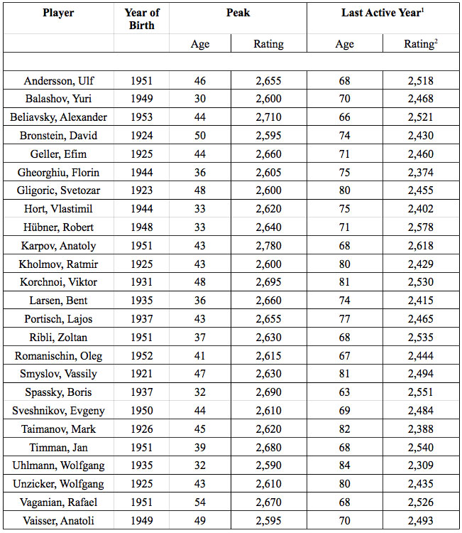
Table 1 shows how ageing has affected the ratings of some former world champions or world class players who are/were active until old age. Jefim Rotstein — who won the German senior championships multiple times — is the only active 2,300+ player, who seems to be immune against ageing. He started at the age of 58 and 2,215 Elo points, reached his peak of 2,418 points at the age of 72, and was rated 2,330 at the age of 86 in January 2020.

Influence of Tournament Activity in Old Age

Vaci et al. (2015) highlighted the benefits of tournament practice in old age. The regression coefficients presented in their Table 2 for their model 1 and in Appendix C for their model 2 could only be replicated if the original databases were used. The original German database lists the number of games per tournament. The authors thus compared hypothetical players who played 3 or 30 games per tournament in their Figure 4 B. There are no tournaments that last for 30 games. The curves were again not symmetric, and fabricated in an unknown way.

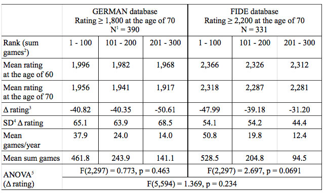
In order to determine the correct influence of tournament practice in old age, all of the FIDE players who had been active at the ages of both 60 and 70 and had reached ≥ 2,200 Elo points at the age of 70 were extracted. Their total number was 331. They were ranked according to the sum of games that they had played during this period, and divided into three groups of ranks 1-100, 101- 200, and 201-300. The same was applied with the 390 German players who had reached 1,800 DWZ (“Deutsche Wertungszahl”, German Evaluation Number) points or more at the age of 70. The rating and games data of the groups are listed in Table 2. The Δ ratings of the groups — defined as the rating differences between the age of 70 and 60 — were compared by ANOVA testing (explained in Table 2). First, there was no significant difference between the FIDE and the German groups when they were tested together, and second, playing more or fewer tournament games did not significantly influence the Δ ratings in both cases. However, in the case of the FIDE groups, the significance limit was only narrowly missed. The Δ rating decreased from -47.99 to -31.2 Elo points if the players were less active and played only 94.5 instead of 528.5 games in the eleven-year period. In other words, FIDE players showed a tendency to benefit from being less active, which

was surprising at first glance. The DWZ system of the German Chess Federation (DSB) is based on the same principles as the FIDE Elo system, although the development coefficients K are different. The higher the K, the more weight that is given to the most recent tournament in the calculation of the new rating value. The FIDE K-values are lower and more conservative than the DSB values. Consequently, FIDE players lag more behind their actual playing strength than German players, and playing less games helps them to preserve their ratings for a longer period.

Discussion

Vaci et al. (2015) went too far in their efforts to prove the validity of Simonton’s (1997) model for chess players. Their paper should not have passed the review process. Peer review is considered the “gold standard” of quality control in science. The former editor of the British Medical Journal (BMJ) — Richard Smith — described this “sacred path” as “slow, expensive, profligate of academic time, highly subjective, something of a lottery, prone to bias, and easily abused” (Smith, 2006). Psychology and Aging and most other peer-reviewed journals ask the authors to suggest their reviewers. Authors usually suggest their friends. Editors can decline the suggestions, but why should they? It is not that easy to find reviewers in specialized fields like chess. I informed Psychology and Aging and the Austrian Agency for Research Integrity (OeAWI) — the authors were employees of the Alpen-Adria University, Klagenfurt, at that time — about this case in 2016. They both acknowledged that my critique was valid. Nevertheless, Vaci, Gula & Bilalić’s (2015) paper continues to mislead its readers more than four years after its publication.

The new RI7 model calculates the overall lifetime trajectory of an unlimited number of chess players in one run with one single function. It avoids the extrapolation error, as well as artefacts due to compositional fallacy. Roring & Charness (2007) fitted their curves piecewise before and after the peak, which was a better option than Vaci et al.’s (2015) approach.

The curves presented in Figure 6 are similar to the composite curves of fluid intelligence (Gf) and crystallized intelligence (Gc) reported in the literature (McArdle, Ferrer-Caja, Hamagami, & Woodcock, 2002). The separation of general intelligence into Gf and Gc is known as the Cattell- Horn-Carroll theory. Gf represents the biological, mostly-inherited part — for example, the processing speed or working memory capacity — whereas Gc is acquired through education and experience. Gf shows a peak in early adulthood, before subsequently steadily declining as a consequence of the influence of ageing on functional neurobiological processes. Instead, Gc increases or remains stable until about the age of 70, when it also starts to decline. Chess intelligence seems to be related to general intelligence, because it shows a similar time course. However, it is not clear at present which of the many abilities summarized under the label general intelligence constitute chess skill. The decline in Gf is compensated by the increase in Gc, whereby chess trajectories are characterized by a long plateau phase after the peak, and a modest decline. There is no inflection point or stabilization in old age, as claimed by Vaci et al. (2015).

The number of tournament games played does not affect the rating in old age because most of the players are either at their performance limit (Howard, 2014) or only playing for entertainment. Only players who have not yet reached their limit — like those who return in middle adulthood after a long period of inactivity — or beginners at any age can benefit from tournament practice.

Players like Korchnoi, Smyslov, and Lasker have demonstrated that ageing has not only a biological but also a psychological or motivational component. German experts are less active in middle and old adulthood, compared with the lower-rated players (see Figure 5). One explanation could be that the most ambitious players tend to lose their motivation when they feel that they have passed their pinnacle and are unable to further improve. The fact that many German players return to tournament chess in old adulthood shows that chess is an attractive hobby not only for the young generation but also for retired persons.

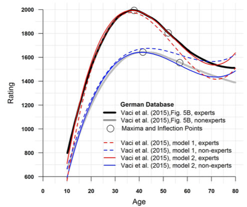
Figure 1. Asymmetric cubic curves. Vaci et al. (2015) marked the peaks and inflection points with small circles, although the corresponding local minima were missing. They eliminated the typical late cubic rise in an unknown way. The actual curves obtained with their models 1 and 2 (blue and red lines) differ from one another, which is explained in Figure 3. The online tool WebplotDigitizer (Ankit Rohatgi, 2019) was used to extract the data points from Vaci et al. (2015), Figure 5 B.

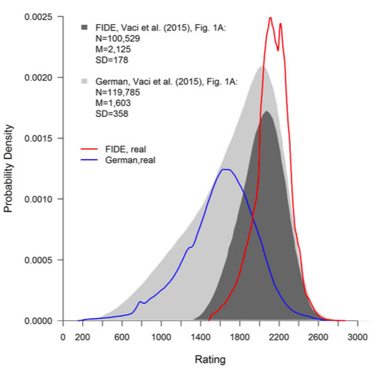
Figure 2. Imaginary probability density curves. Vaci et al.’s (2015) density curves were fabricated in an unknown way. The area under the curve – expressed as percentages – indicates the probability of finding observations within a specific range of ratings. The red and blue lines show the correct curves. The online tool WebplotDigitizer (Rohatgi, 2019) was used to extract the data points from Vaci et al. (2015), Figure 1 A.

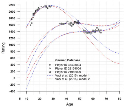
Figure 3. Extrapolation error in Vaci et al.’s (2015) models. Chess players’ activity periods are rather short. The missing data are estimated by extrapolation. Long- distance extrapolation leads to unrealistic values, which is demonstrated by the example of three German players. The authors’ models 1 and 2 produced different extrapolations, which explains the different curves in Figure 1.

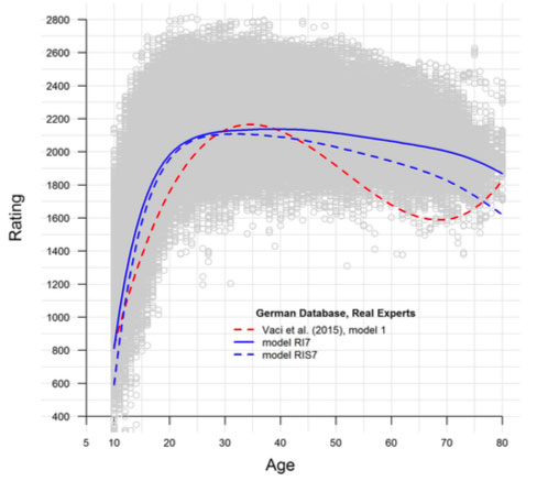
Figure 4. Correct RI7 model. The 398,643 observations of the 12,535 real German experts form a grey cloud. The overall curve obtained with Vaci et al.’s (2015) model 1 (red dashed line) is outside the cloud from about 55 years of age onwards, and thus drastically incorrect. The RIS7 model (blue, dashed line) also suffers from extrapolation error, while the RI7 model (blue, solid line) does not.

RI7 = polynomial 7th degree and random intercept
RIS7 = polynomial 7th degree and random intercept combined with random slope

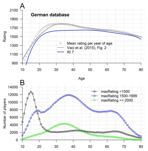
Figure 5. Compositional fallacy. Vaci et al.’s (2015) loess curve – presented in their Figure 2, is reproduced as a grey line in Figure A. It mirrors the mean ratings per year (grey circles). Figure B shows that differently-skilled players are active at different times. The RI7 curve (blue line) in Figure A controls for this artefact, which Simonton (1997) dubbed as a “compositional fallacy”.

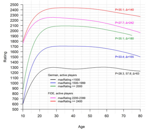
Figure 6. Trajectories of differently-skilled FIDE and German players. Below- average German players (black line) are the only group who show a second peak at around 58 years of age. Age is kindest to them. The lower-skilled FIDE players (magenta line) decline faster after the peak, which is probably an artefact (see ‘Lifetime Trajectories of FIDE and German Players’ section). In the case of the German experts (≥ 2,000 points), the number of active players dropped below 50 at the age of 77, whereby only the period from 10 to 75 years was monitored. (Active = games > 0 at each listing. P = age at peak. Δ = rating difference between the peak and the age of 75).

Table 1: Comparison of some former world champions’ and world-class players’ peak ratings, with their ratings in their last active year until 2019.

¹ active = games played per year > 0

² mean rating per year

Table 2: Influence of tournament practice on the ratings of FIDE and German players who were active at 60 as well as 70 years of age.

¹ Number of players
² Sum of games played in the period from 60 to 70 years of age

³ Rating at the age of 70 minus rating at the age of 60
⁴ Standard deviation

⁵ Analysis of variance. The F-value is the quotient of the between-group and the within-group variance. It depends on the degrees of freedom given in the brackets, which indicate how many groups and how many players are analysed. The p-value gives the probability that the calculated F- value is actually observed. If the p-value is less than 0.05 – which corresponds to an uncertainty of below 5 % - the difference between the tested groups is generally accepted as being statistically significant.

References

Ankit Rohatgi, WebPlotDigitizer Version: 4.2, April, 2019.
Bates D., Maechler M., Bolker B., & Walker S. (2015). Fitting Linear Mixed-Effects Models Using
lme4. Journal of Statistical Software, 67(1), 1-48.
Bilalic, M., Smallbone, K., McLeod, P., & Gobet, F. (2009). Why are (the best) women so good at chess? Participation rates and gender differences in intellectual domains. Proceedings Biological Sciences, 276, 1161-1165.
Bartelski, W. (2019), OlimpBase, Elo lists 1971-2001
Elo, A. E. (2008). The Rating of Chessplayers, Past & Present. Bronx, NY: Ishi Press International.
(originally published in 1978)
Howard, R. W. (2006). A complete database of international chess players and chess performance ratings for varied longitudinal studies. Behav. Res. Methods 38, 698–703.
Howard, R. W. (2014). Gender differences in intellectual performance persist at the limits of individual capabilities. Journal of Biosocial Science, 46, 386-404.
McArdle, J. J., Ferrer-Caja, E., Hamagami, F. & Woodcock, R. W. (2002). Comparative longitudinal structural analyses of the growth and decline of multiple intellectual abilities over the life span. Developmental Psychology, 38, 115-142.
Open Science Collaboration (2015), Estimating the reproducibility of psychological science. Science. Vol. 349, Issue 6251, aac4716
R Core Team. (2015). R: A Language and environment for statistical computing. Vienna, Austria: R Foundation for Statistical Computing. Retrieved from http://www.R-project.org/
Roring, R. W., & Charness, N. (2007). A multilevel model analysis of expertise in chess across the 24 life span. Psychology and Aging, 22, 291-299,
Simonton, D. K. (1997). Creative productivity: A predictive and explanatory model of career trajectories and landmarks. Psychological Review, 104, 66-89.
Smith, R. (2006). Peer review: a flawed process at the heart of science and journals. J R Soc Med 2006;99:178–182
Vaci, N., Gula, B., & Bilalić, M. (2014). Restricting range restricts conclusions. Frontiers in Psychology, 5, 569.
Vaci, N., Gula, B., & Bilalić, M. (2015). Is Age Really Cruel to Experts? Compensatory Effects of Activity. Psychology and Aging, 30, 740-754.
Vaci, N. , Bilalic ́ M. (2017). Chess databases as a research vehicle in psychology: Modeling large data. Behav. Res. Methods 49, 1227–1240 (2017).
Wiesend B. (2019), Questioning Gender Studies on Chess, Chessbase News